5. Connecting with accounting databases

5.1. Power BI

The easiest way to exploit the Python ecosystem in Power BI is to enable Python scripting inside Power BI. For that, you need to have Python installed in your system.

In Power BI, check from Options - Global - Python scripting that you have correct folders for your Python and IDE. Power BI should detect the folders automatically, but it is good to check.

Furthermore, you need to have at least Pandas, Matplotlib and Numpy installed.

You can run Python scripts inside Power BI using Get Data - Other - Python script. However, it is a good habit to check in your Python environment that the script is working.

There are a few limitations with the connection between Power BI/Python:

• If you want to import data, it should be represented in a Pandas data frame.

• The maximum run time of a script is 30 minutes.

• You must use full directory paths in your code, not relative paths.

• Nested tables are not supported.

Otherwise, implementing Python in Power BI is very similar to doing analysis purely inside Python. The good thing is, of course, that you have the tools of both Python and Power BI at your disposal.

5.2. MySQL, SAP and others

There are good libraries for connecting to MySQL, for example, MySQLdb: pypi.org/project/MySQL-python/. If you want, you can use your MySQL database to go through the examples, instead of SQlite.

SAP HANA is used to connect with Python to a SAP database. Here are the instructions on how to connect Python to SAP: developers.sap.com/tutorials/hana-clients-python.html. The task is quite difficult, and we are not doing that in this course.

5.3. Sqlite

In the following, we will analyse our example database purely in Python. For that, we use an example company database that is available here: github.com/jpwhite3/northwind-SQLite3

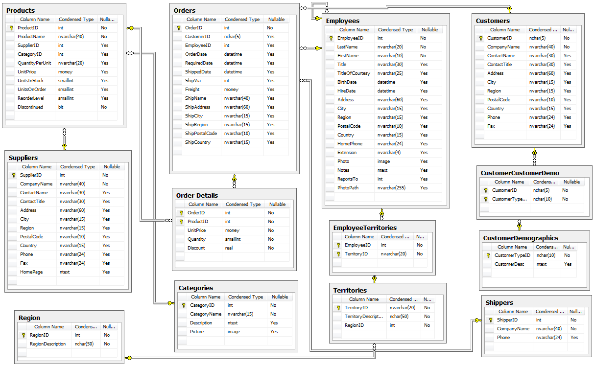
This demo-database has originally been published to Microsoft Access 2000. We analyse it using Sqlite3. However, keep in mind that you can repeat the following analysis by connecting to many other databases, like SAP. In the following, we use some basic SQL statements. However, this course is not about SQL, so we do not go deeper in that direction.

Sqlite3 is included in the standard library. So, you do not need to install any additional libraries. Let’s start by importing the library.

import sqlite3

We can create a connection to the example database with connect(). You need to have the Northwind_large.sqlite file in your work folder for the following command to work.

connection = sqlite3.connect('Northwind_large.sqlite')

cursor() returns a cursor for the connection. A cursor -object has many useful methods to execute SQL statements.

cursor = connection.cursor()

The tables of the database can be collected with the following commands. execute() is used for a SQL statement and fetchall() collects all the rows from the result.

cursor.execute("SELECT name FROM sqlite_master WHERE type='table'")
print(cursor.fetchall())

[('Employees',), ('Categories',), ('Customers',), ('Shippers',), ('Suppliers',), ('Orders',), ('Products',), ('OrderDetails',), ('CustomerCustomerDemo',), ('CustomerDemographics',), ('Region',), ('Territories',), ('EmployeeTerritories',)]

We check the fields of the Employees, OrderDetails, Orders and Products tables. The outpus are messy lists of tuples. The name of a field is always the second item in a tuple.

cursor.execute("PRAGMA table_info(Employees)")
print(cursor.fetchall())

[(0, 'Id', 'INTEGER', 0, None, 1), (1, 'LastName', 'VARCHAR(8000)', 0, None, 0), (2, 'FirstName', 'VARCHAR(8000)', 0, None, 0), (3, 'Title', 'VARCHAR(8000)', 0, None, 0), (4, 'TitleOfCourtesy', 'VARCHAR(8000)', 0, None, 0), (5, 'BirthDate', 'VARCHAR(8000)', 0, None, 0), (6, 'HireDate', 'VARCHAR(8000)', 0, None, 0), (7, 'Address', 'VARCHAR(8000)', 0, None, 0), (8, 'City', 'VARCHAR(8000)', 0, None, 0), (9, 'Region', 'VARCHAR(8000)', 0, None, 0), (10, 'PostalCode', 'VARCHAR(8000)', 0, None, 0), (11, 'Country', 'VARCHAR(8000)', 0, None, 0), (12, 'HomePhone', 'VARCHAR(8000)', 0, None, 0), (13, 'Extension', 'VARCHAR(8000)', 0, None, 0), (14, 'Photo', 'BLOB', 0, None, 0), (15, 'Notes', 'VARCHAR(8000)', 0, None, 0), (16, 'ReportsTo', 'INTEGER', 0, None, 0), (17, 'PhotoPath', 'VARCHAR(8000)', 0, None, 0)]

cursor.execute("PRAGMA table_info(OrderDetails)")
print(cursor.fetchall())

[(0, 'Id', 'VARCHAR(8000)', 0, None, 1), (1, 'OrderId', 'INTEGER', 1, None, 0), (2, 'ProductId', 'INTEGER', 1, None, 0), (3, 'UnitPrice', 'DECIMAL', 1, None, 0), (4, 'Quantity', 'INTEGER', 1, None, 0), (5, 'Discount', 'DOUBLE', 1, None, 0)]

cursor.execute("PRAGMA table_info(Orders)")
print(cursor.fetchall())

[(0, 'Id', 'INTEGER', 0, None, 1), (1, 'CustomerId', 'VARCHAR(8000)', 0, None, 0), (2, 'EmployeeId', 'INTEGER', 1, None, 0), (3, 'OrderDate', 'VARCHAR(8000)', 0, None, 0), (4, 'RequiredDate', 'VARCHAR(8000)', 0, None, 0), (5, 'ShippedDate', 'VARCHAR(8000)', 0, None, 0), (6, 'ShipVia', 'INTEGER', 0, None, 0), (7, 'Freight', 'DECIMAL', 1, None, 0), (8, 'ShipName', 'VARCHAR(8000)', 0, None, 0), (9, 'ShipAddress', 'VARCHAR(8000)', 0, None, 0), (10, 'ShipCity', 'VARCHAR(8000)', 0, None, 0), (11, 'ShipRegion', 'VARCHAR(8000)', 0, None, 0), (12, 'ShipPostalCode', 'VARCHAR(8000)', 0, None, 0), (13, 'ShipCountry', 'VARCHAR(8000)', 0, None, 0)]

cursor.execute("PRAGMA table_info(Products)")
print(cursor.fetchall())

[(0, 'Id', 'INTEGER', 0, None, 1), (1, 'ProductName', 'VARCHAR(8000)', 0, None, 0), (2, 'SupplierId', 'INTEGER', 1, None, 0), (3, 'CategoryId', 'INTEGER', 1, None, 0), (4, 'QuantityPerUnit', 'VARCHAR(8000)', 0, None, 0), (5, 'UnitPrice', 'DECIMAL', 1, None, 0), (6, 'UnitsInStock', 'INTEGER', 1, None, 0), (7, 'UnitsOnOrder', 'INTEGER', 1, None, 0), (8, 'ReorderLevel', 'INTEGER', 1, None, 0), (9, 'Discontinued', 'INTEGER', 1, None, 0)]

Pandas has a very convenient function, read_sql_query, to load SQL queries to dataframes. Let’s start by loading Pandas.

import pandas as pd

SQL queries are a whole new world, and we use only the essential. The following code picks up LastName from the Employees table, UnitPrice and Quantity from the OrderDetails, OrderDate and ShipCountry from Orders, CategoryName from Categories, and ProductName from Products. The next part of the code is important. The JOIN commands connect the data in different tables in a correct way. Notice how we qive our sqlite3 database connection -object as a paramter to the function.

query_df = pd.read_sql_query("""SELECT Employees.LastName, OrderDetails.UnitPrice, 
OrderDetails.Quantity, Orders.OrderDate, Orders.ShipCountry, Categories.CategoryName, Products.ProductName
FROM OrderDetails
JOIN Orders ON Orders.Id=OrderDetails.OrderID
JOIN Employees ON Employees.Id=Orders.EmployeeId
JOIN Products ON Products.ID=OrderDetails.ProductId
JOIN Categories ON Categories.ID=Products.CategoryID""", connection)

query_df

	LastName	UnitPrice	Quantity	OrderDate	ShipCountry	CategoryName	ProductName
0	Buchanan	14.00	12	2012-07-04	France	Dairy Products	Queso Cabrales
1	Buchanan	9.80	10	2012-07-04	France	Grains/Cereals	Singaporean Hokkien Fried Mee
2	Buchanan	34.80	5	2012-07-04	France	Dairy Products	Mozzarella di Giovanni
3	Suyama	18.60	9	2012-07-05	Germany	Produce	Tofu
4	Suyama	42.40	40	2012-07-05	Germany	Produce	Manjimup Dried Apples
...	...	...	...	...	...	...	...
621878	Davolio	21.00	20	2013-08-31 02:59:28	Venezuela	Grains/Cereals	Gustaf's Knäckebröd
621879	Davolio	13.00	11	2013-08-31 02:59:28	Venezuela	Condiments	Original Frankfurter grüne Soße
621880	Davolio	39.00	45	2013-08-31 02:59:28	Venezuela	Meat/Poultry	Alice Mutton
621881	Davolio	25.00	7	2013-08-31 02:59:28	Venezuela	Condiments	Grandma's Boysenberry Spread
621882	Davolio	21.05	27	2013-08-31 02:59:28	Venezuela	Condiments	Louisiana Fiery Hot Pepper Sauce

621883 rows × 7 columns

Now that we have everything neatly in a Pandas dataframe, we can do many kinds of analyses. The other chapters focus more on the Pandas functionality, but let’s try something that we can do.

For example, to analyse trends, we can change OrderDate to a datetime object with to_datetime().

query_df['OrderDate'] = pd.to_datetime(query_df['OrderDate'])

query_df

	LastName	UnitPrice	Quantity	OrderDate	ShipCountry	CategoryName	ProductName
0	Buchanan	14.00	12	2012-07-04 00:00:00	France	Dairy Products	Queso Cabrales
1	Buchanan	9.80	10	2012-07-04 00:00:00	France	Grains/Cereals	Singaporean Hokkien Fried Mee
2	Buchanan	34.80	5	2012-07-04 00:00:00	France	Dairy Products	Mozzarella di Giovanni
3	Suyama	18.60	9	2012-07-05 00:00:00	Germany	Produce	Tofu
4	Suyama	42.40	40	2012-07-05 00:00:00	Germany	Produce	Manjimup Dried Apples
...	...	...	...	...	...	...	...
621878	Davolio	21.00	20	2013-08-31 02:59:28	Venezuela	Grains/Cereals	Gustaf's Knäckebröd
621879	Davolio	13.00	11	2013-08-31 02:59:28	Venezuela	Condiments	Original Frankfurter grüne Soße
621880	Davolio	39.00	45	2013-08-31 02:59:28	Venezuela	Meat/Poultry	Alice Mutton
621881	Davolio	25.00	7	2013-08-31 02:59:28	Venezuela	Condiments	Grandma's Boysenberry Spread
621882	Davolio	21.05	27	2013-08-31 02:59:28	Venezuela	Condiments	Louisiana Fiery Hot Pepper Sauce

621883 rows × 7 columns

Next, we can change our datetime object as index.

query_df.index = query_df['OrderDate']

query_df

	LastName	UnitPrice	Quantity	OrderDate	ShipCountry	CategoryName	ProductName
OrderDate
2012-07-04 00:00:00	Buchanan	14.00	12	2012-07-04 00:00:00	France	Dairy Products	Queso Cabrales
2012-07-04 00:00:00	Buchanan	9.80	10	2012-07-04 00:00:00	France	Grains/Cereals	Singaporean Hokkien Fried Mee
2012-07-04 00:00:00	Buchanan	34.80	5	2012-07-04 00:00:00	France	Dairy Products	Mozzarella di Giovanni
2012-07-05 00:00:00	Suyama	18.60	9	2012-07-05 00:00:00	Germany	Produce	Tofu
2012-07-05 00:00:00	Suyama	42.40	40	2012-07-05 00:00:00	Germany	Produce	Manjimup Dried Apples
...	...	...	...	...	...	...	...
2013-08-31 02:59:28	Davolio	21.00	20	2013-08-31 02:59:28	Venezuela	Grains/Cereals	Gustaf's Knäckebröd
2013-08-31 02:59:28	Davolio	13.00	11	2013-08-31 02:59:28	Venezuela	Condiments	Original Frankfurter grüne Soße
2013-08-31 02:59:28	Davolio	39.00	45	2013-08-31 02:59:28	Venezuela	Meat/Poultry	Alice Mutton
2013-08-31 02:59:28	Davolio	25.00	7	2013-08-31 02:59:28	Venezuela	Condiments	Grandma's Boysenberry Spread
2013-08-31 02:59:28	Davolio	21.05	27	2013-08-31 02:59:28	Venezuela	Condiments	Louisiana Fiery Hot Pepper Sauce

621883 rows × 7 columns

We still need to order the index.

query_df.sort_index(inplace=True)

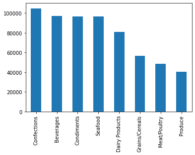
Let’s calculate the total number of orders for different product categories.

query_df['CategoryName'].value_counts().plot.bar()

<AxesSubplot:>

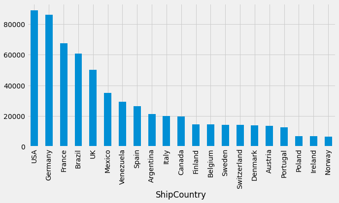
Let’s check next, to which country the company is selling the most. The following command is quite long! First, it groups values by ShipCountry, then counts values and sorts them in a descending order by Quantity, and finally selects only Quantity -column.

query_df.groupby('ShipCountry').count().sort_values('Quantity',ascending=False)['Quantity']

ShipCountry
USA            89059
Germany        85923
France         67314
Brazil         60663
UK             50162
Mexico         34979
Venezuela      29128
Spain          26270
Argentina      21233
Italy          19952
Canada         19652
Finland        14661
Belgium        14505
Sweden         14147
Switzerland    14049
Denmark        13764
Austria        13669
Portugal       12684
Poland          6756
Ireland         6688
Norway          6625
Name: Quantity, dtype: int64

A nice thing in Python (and Pandas) is that we change the previous to a bar chart just by adding plot.bar() to the end of the command.

Let’s first load Matplotlib to make our plots prettier.

import matplotlib.pyplot as plt

plt.style.use('fivethirtyeight')

query_df.groupby('ShipCountry').count().sort_values('Quantity',ascending=False)['Quantity'].plot.bar(figsize=(10,5))
plt.show()

With pivot tables, we can do a 2-way grouping.

query_df.pivot_table(index='LastName',columns='ShipCountry',values='Quantity',aggfunc=sum)

ShipCountry	Argentina	Austria	Belgium	Brazil	Canada	Denmark	Finland	France	Germany	Ireland	...	Mexico	Norway	Poland	Portugal	Spain	Sweden	Switzerland	UK	USA	Venezuela
LastName
Buchanan	68252	40687	45468	182595	55898	47414	40935	169200	265031	21996	...	103888	18487	19077	34787	76052	46805	39866	123721	263998	95810
Callahan	50977	46506	21741	201153	58506	42306	27732	192488	237532	16133	...	86354	12045	19728	31522	73022	40745	34171	155124	250614	62389
Davolio	66186	44332	47841	150727	50957	42275	47406	186479	229137	16471	...	105282	9071	22855	31563	61587	33431	38221	149707	258013	73040
Dodsworth	48936	42499	45385	173881	58663	29649	38434	218987	239419	23881	...	91115	16886	19259	43262	69528	36657	50513	146315	207208	105907
Fuller	61848	25092	46255	155750	55919	29790	30799	184553	228026	20975	...	119410	22544	21392	30644	69067	31062	31412	130891	250988	86679
King	45559	39419	41950	166678	45888	31635	56539	194100	258696	15336	...	94927	35009	16933	28930	62777	46751	43769	162153	240532	74124
Leverling	64409	38191	35325	188315	74915	36741	42688	204843	243401	22365	...	82019	21029	13554	39832	82488	46028	44096	146039	305553	66031
Peacock	62869	28476	52329	171980	56217	46333	50386	172114	244482	12059	...	89564	18977	12986	44000	92110	40524	44052	132325	252295	90487
Suyama	69697	44687	35595	148480	45064	43631	39998	193725	246849	22518	...	123194	14638	24995	37539	82311	38743	31109	134042	246389	87347

9 rows × 21 columns

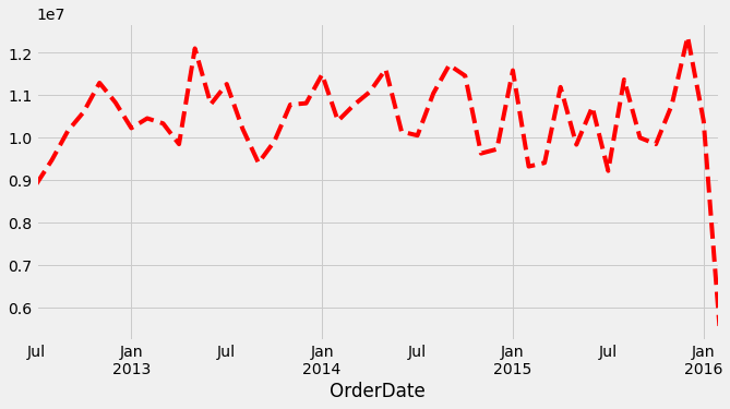
With Quantity and OrderPrice, we can calculate the total price of the orders. Using * for multiplication, Python/Pandas makes the multiplication element-wise.

query_df['TotalPrice'] = query_df['Quantity']*query_df['UnitPrice']

There is too much information to one plot, so let’s resample the data before plotting (‘M’ means monthly).

query_df['TotalPrice'].resample('M').sum().plot(figsize=(10,5),style='r--')

<AxesSubplot:xlabel='OrderDate'>

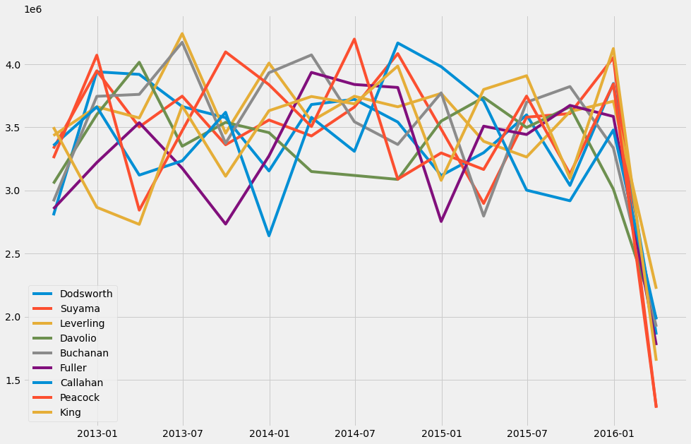
Let’s plot how the sales of different salesperson have progressed. The for loop in the command goes through all the salesperson and draws their performance to the same chart. With set, we can pick from the LastName column unique values.

plt.figure(figsize=(15,10))
for name in set(query_df['LastName']):
    plt.plot(query_df['TotalPrice'][query_df['LastName'] == name].resample('Q').sum())
plt.legend(set(query_df['LastName']))
plt.show()

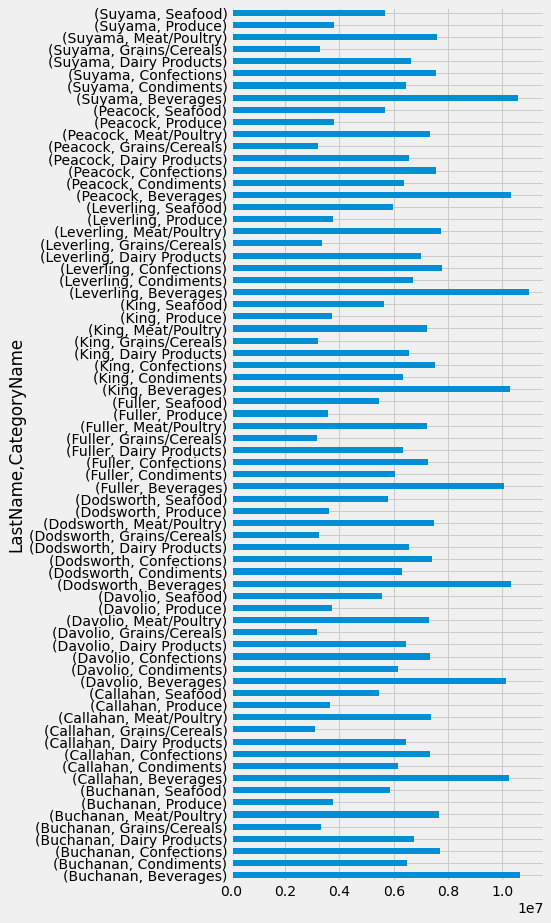
We can also use bar charts. Here are the sales of different salesperson and product categories. We first do a two-level grouping, sum the values in those groups, and pick TotalPrice. Adding plot.barh() to the end turns the 2-level grouping table into a bar chart.

query_df.groupby(['LastName','CategoryName']).sum()['TotalPrice'].plot.barh(figsize=(5,15))
plt.show()

We can also use percentage values in tables. (I admit, the following command is a mess!). It divides the values of a LastName/CategoryName -pivot table with the row sums of that table. Then, it multiplies these numbers by hundred. style.format is used to decrease the number of decimals to 2 2f, and to add % to the end.

(query_df.pivot_table(values = 'TotalPrice', index = 'LastName',
                      columns = 'CategoryName').divide(query_df.pivot_table(values = 'TotalPrice',
                    index = 'LastName', columns = 'CategoryName').sum(axis=1),axis=0)*100).style.format('{:.2f} %')

CategoryName	Beverages	Condiments	Confections	Dairy Products	Grains/Cereals	Meat/Poultry	Produce	Seafood
LastName
Buchanan	15.70 %	9.51 %	10.41 %	11.92 %	8.35 %	22.39 %	13.14 %	8.58 %
Callahan	15.71 %	9.52 %	10.41 %	11.84 %	8.18 %	22.45 %	13.44 %	8.45 %
Davolio	15.45 %	9.46 %	10.37 %	11.89 %	8.34 %	22.36 %	13.70 %	8.43 %
Dodsworth	15.65 %	9.64 %	10.32 %	11.91 %	8.38 %	22.36 %	13.06 %	8.67 %
Fuller	15.73 %	9.45 %	10.39 %	11.87 %	8.39 %	22.35 %	13.28 %	8.53 %
King	15.59 %	9.59 %	10.56 %	11.94 %	8.36 %	21.95 %	13.49 %	8.53 %
Leverling	15.69 %	9.58 %	10.42 %	11.98 %	8.37 %	22.31 %	13.08 %	8.58 %
Peacock	15.41 %	9.50 %	10.44 %	11.83 %	8.33 %	22.27 %	13.61 %	8.60 %
Suyama	15.63 %	9.52 %	10.36 %	11.86 %	8.34 %	22.40 %	13.38 %	8.52 %

5.4. Other sources of accounting data

Google Dataset Search is an excellent source of datasets, including interesting accounting datasets: datasetsearch.research.google.com/

Quandl is another interesting source of data. They have some free datasets, but you need to register to get an api key before you can download any data. Quandl offers a library that you can use to download datasets directly in Python: www.quandl.com/

5.4.1. Pandas Datareader

Pandas Datareader is a library that can be used to download external datasets to Pandas dataframes. pandas-datareader.readthedocs.io/en/latest/

Currently, the following sources are supported in Pandas Datareader

• Tiingo

• IEX

• Alpha Vantage

• Enigma

• EconDB

• Quandl

• St.Louis FED (FRED)

• Kenneth French’s data library

• World Bank

• OECD

• Eurostat

• Thrift Savings Plan

• Nasdaq Trader symbol definitions

• Stooq

• MOEX

• Naver Finance

For most of these, free registration is required to get an API key.

You need to install Datareader first. It is included in Anaconda and can also be installed with Pip using a command pip install pandas-datareader.

Let’s import the library

import pandas_datareader as pdr

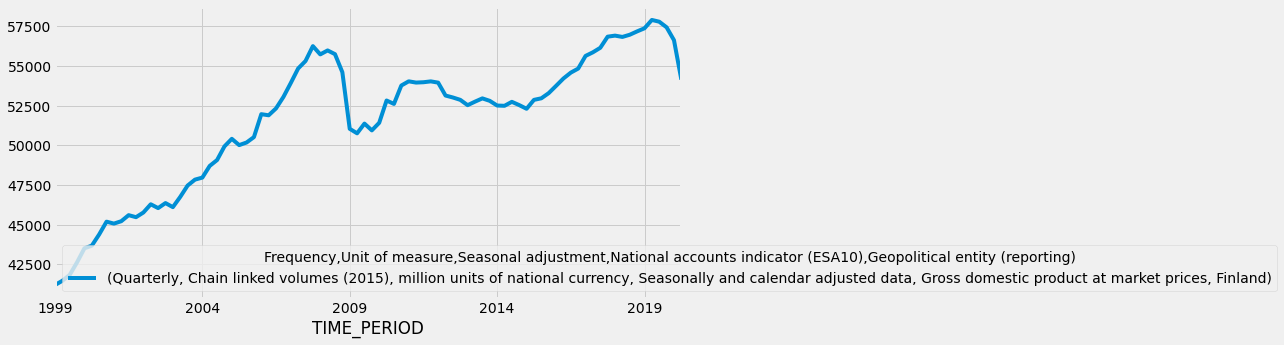
Let’s use in our example EconDB (www.econdb.com/). In the following code, we load the quarterly values of Finland’s gross domectic product from the year 1999 to the most recent value.

data = pdr.data.DataReader('ticker=RGDPFI','econdb',start=1999)

It returns a Pandas dataframe, to which we can apply all the Pandas functions.

data.plot(figsize=(10,5))
plt.show()

Fama/French data library is also very interesting for accounting research. mba.tuck.dartmouth.edu/pages/faculty/ken.french/data_library.html

import pandas_datareader.famafrench as fama

There are 297 datasets available.

len(fama.get_available_datasets())

297

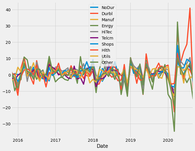
Let’s load an industry portfolio return data.

data2 = pdr.data.DataReader('10_Industry_Portfolios', 'famafrench')

This time, it returns a dictionary. The items of the dictionary are dataframes with different data. DESCR can be used to get information about the data.

type(data2)

dict

data2['DESCR']

'10 Industry Portfolios\n----------------------\n\nThis file was created by CMPT_IND_RETS using the 202009 CRSP database. It contains value- and equal-weighted returns for 10 industry portfolios. The portfolios are constructed at the end of June. The annual returns are from January to December. Missing data are indicated by -99.99 or -999. Copyright 2020 Kenneth R. French\n\n  0 : Average Value Weighted Returns -- Monthly (59 rows x 10 cols)\n  1 : Average Equal Weighted Returns -- Monthly (59 rows x 10 cols)\n  2 : Average Value Weighted Returns -- Annual (5 rows x 10 cols)\n  3 : Average Equal Weighted Returns -- Annual (5 rows x 10 cols)\n  4 : Number of Firms in Portfolios (59 rows x 10 cols)\n  5 : Average Firm Size (59 rows x 10 cols)\n  6 : Sum of BE / Sum of ME (6 rows x 10 cols)\n  7 : Value-Weighted Average of BE/ME (6 rows x 10 cols)'

data2[0].plot(figsize=(10,8))

<AxesSubplot:xlabel='Date'>