2. NLP example - LDA and other summarisation tools
In this example, we analyse a collection of academic journals with Latent Dirichlet Allocation (LDA) and other summarisation tools.
To manipulate and list files in directories, we need the os -library.
import os
I have the data in the acc_journals -folder that is under the work folder. Unfortunately, this data is not available anywhere. If you want to follow this example, just put a collection of txt-files to a “acc_journals”-folder (under the work folder) and follow the steps.
data_path = './acc_journals/'
listdir() makes a list of filenames inside data_path
files = os.listdir(data_path)
The name of the first text file is “2019_1167.txt”.
files[0]
'2019_1167.txt'
In total, we have 2126 articles.
len(files)
2126
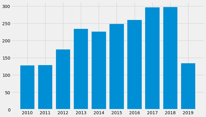
The filenames have a publication year as the first four digits of the name. With the following code we can collect the publication years to a list.
file_years = []
for file in files:
    file_years.append(int(file[:4])) # Pick the first four letters from the filename -string and turn it into a integer.
[file_years.count(a) for a in set(file_years)]
[260, 296, 297, 134, 128, 129, 174, 234, 226, 248]
In this example we will need numpy to manipulate arrays, and Matplotlib for plots.
import numpy as np
import matplotlib.pyplot as plt
Let’s plot the number of documents per year.
plt.style.use('fivethirtyeight') # Define the style of figures.
plt.figure(figsize=[10,6]) # Define the size of figures.
# The first argument: years, the second argument: the list of document frequencies for different years (built using list comprehension)
plt.bar(list(set(file_years)),[file_years.count(a) for a in set(file_years)])
plt.xticks(list(set(file_years))) # The years below the bars
plt.show()
The common practice is to remove stopwords from documents. These are common fill words that do not contain information about the content of documents. We use the stopwords-list from the NLTK library (www.nltk.org). Here is a short description of NLTK from their web page: “NLTK is a leading platform for building Python programs to work with human language data. It provides easy-to-use interfaces to over 50 corpora and lexical resources such as WordNet, along with a suite of text processing libraries for classification, tokenization, stemming, tagging, parsing, and semantic reasoning, wrappers for industrial-strength NLP libraries, and an active discussion forum.”
from nltk.corpus import stopwords
stop_words = stopwords.words("english")
Here are some example stopwords.
stop_words[0:10]
['i', 'me', 'my', 'myself', 'we', 'our', 'ours', 'ourselves', 'you', "you're"]
Usually, stopword-lists are extended with useless words specific to the corpus we are analysing. That is done below. These additional words are found by analysing the results at different steps of the analysis. Then the analysis is repeated.
stop_words.extend(['fulltext','document','downloaded','download','emerald','emeraldinsight',
                   'accepted','com','received','revised','archive','journal','available','current',
                   'issue','full','text','https','doi','org','www','com''ieee','cid','et','al','pp',
                   'vol','fig','reproduction','prohibited','reproduced','permission','accounting','figure','chapter'])
The following code reads every file in the files list and reads it content as an item to the raw_text list. Thus, we have a list with 2126 items and where each item is a raw text of one document.
raw_text = []
for file in files:
    fd = open(os.path.join(data_path,file),'r',errors='ignore')
    raw_text.append(fd.read())
Here is an example of raw text from the first document.
raw_text[0][3200:3500]
'currency exchanges and markets have daily dollar volume of around $50 billion.1 Over 300 "cryptofunds" have emerged (hedge funds that invest solely in cryptocurrencies), attracting around $10 billion in assets under management (Rooney and Levy 2018).2 Recently, bitcoin futures have commenced trading'
For the following steps, we need Gensim that is a multipurpose NLP library especially designed for topic modelling.
Here is a short description from the Gensim Github-page (github.com/RaRe-Technologies/gensim):
“Gensim is a Python library for topic modelling, document indexing and similarity retrieval with large corpora. Target audience is the natural language processing (NLP) and information retrieval (IR) community. Features:
All algorithms are memory-independent w.r.t. the corpus size (can process input larger than RAM, streamed, out-of-core),
Intuitive interfaces
Easy to plug in your own input corpus/datastream (trivial streaming API)
Easy to extend with other Vector Space algorithms (trivial transformation API)
Efficient multicore implementations of popular algorithms, such as online Latent Semantic Analysis (LSA/LSI/SVD), Latent Dirichlet Allocation (LDA), Random Projections (RP), Hierarchical Dirichlet Process (HDP) or word2vec deep learning.
Distributed computing: can run Latent Semantic Analysis and Latent Dirichlet Allocation on a cluster of computers.”
import gensim
Gensim has a convenient simple_preprocess() -function that makes many text cleaning procedures automatically. It converts a document into a list of lowercase tokens, ignoring tokens that are too short (less than two characters) or too long (more than 15 characters). The following code goes through all the raw texts and applies simple_preprocess() to them. So, docs_cleaned is a list with lists of tokens as items.
docs_cleaned = []
for item in raw_text:
    tokens = gensim.utils.simple_preprocess(item)
    docs_cleaned.append(tokens)
Here is an example from the first document after cleaning. The documents are now lists of tokens, and here the list is joined back as a string of text.
" ".join(docs_cleaned[0][300:400])
'for assistance relating to data acknowledges financial support from the capital markets co operative research centre acknowledges financial support from the australian research council arc de supplementary data can be found on the review of financial studies web site send correspondence to talis putnins uts business school university of technology sydney po box broadway nsw australia telephone mail talis putnins uts edu au the author published by oxford university press on behalf of the society for financial studies all rights reserved for permissions please mail journals permissions oup com doi rfs hhz downloaded from https academic oup com rfs article'
Next, we remove the stopwords from the documents.
docs_nostops = []
for item in docs_cleaned:
    red_tokens = [word for word in item if word not in stop_words]
    docs_nostops.append(red_tokens)
An example text from the first document after removing the stopwords.
" ".join(docs_nostops[0][300:400])
'hedge funds invest solely attracting around billion assets management rooney levy recently bitcoin futures commenced trading cme cboe catering institutional demand trading hedging bitcoin fringe asset quickly maturing rapid growth anonymity provide users created considerable regulatory challenges application million cryptocurrency exchange traded fund etf rejected securities exchange commission sec march several rejected amid concerns including lack regulation chinese government banned residents trading made initial coin offerings icos illegal september central bank heads bank england mark carney publicly expressed concerns many potential benefits including faster efficient settlement payments regulatory concerns center around use illegal trade drugs hacks thefts illegal pornography even'
As a next step, we remove everything else but nouns, adjectives, verbs and adverbs recognised by our language model. As our language model, we use the large English model from Spacy (spacy.io). Here are some key features of Spacy from their web page:
Non-destructive tokenisation
Named entity recognition
Support for 59+ languages
46 statistical models for 16 languages
Pretrained word vectors
State-of-the-art speed
Easy deep learning integration
Part-of-speech tagging
Labelled dependency parsing
Syntax-driven sentence segmentation
Built-in visualisers for syntax and NER
Convenient string-to-hash mapping
Export to NumPy data arrays
Efficient binary serialisation
Easy model packaging and deployment
Robust, rigorously evaluated accuracy
First, we load the library.
import spacy
Then we define that only certain part-of-speed (POS) -tags are allowed.
allowed_postags=['NOUN', 'ADJ', 'VERB', 'ADV']
The en_core_web_lg model is quite large (700MB) so it takes a while to download it. We do not need the dependency parser or named-entity-recognition, so we disable them.
nlp = spacy.load('en_core_web_lg', disable=['parser', 'ner'])
The following code goes through the documents and removes words that are not recognised by our language model as nouns, adjectives, verbs or adverbs.
docs_lemmas = []
for red_tokens in docs_nostops:
    doc = nlp(" ".join(red_tokens)) # We need to join the list of tokens back to a single string.
    docs_lemmas.append([token.lemma_ for token in doc if token.pos_ in allowed_postags])
Here is again an example text from the first document. Things are looking good. We have a clean collection of words that are meaningful when we try to figure out what is discussed in the text.
" ".join(docs_lemmas[0][300:400])
'silk road marketplace combine public nature blockchain provide unique laboratory analyze illegal ecosystem evolve bitcoin network individual identity mask pseudo anonymity character alpha public nature blockchain allow link bitcoin transaction individual user market participant identify user release see next autonomous future commence trade contract bitcoin price approximately bitcoin time future launch contract notional value academic library user review financial study seize authority bitcoin seizure combine source provide sample user know involved illegal activity starting point analysis apply different empirical approach go sample estimate population illegal activity first approach exploit trade network user know involve illegal activity illegal user use bitcoin'
Next, we build our bigram-model. Bigrams are two-word pairs that naturally belong together. Like the words New and York. We connect these words before we do the LDA analysis.
bigram = gensim.models.Phrases(docs_lemmas,threshold = 80, min_count=3)
bigram_mod = gensim.models.phrases.Phraser(bigram)
docs_bigrams = [bigram_mod[doc] for doc in docs_lemmas]
In this sample text, the model creates bigrams academic_library, starting_point and bitcoin_seizure. The formed bigrams are quite good. It is very often difficult to set the parameters of Phrases so that we have only reasonable bigrams.
" ".join(docs_bigrams[0][300:400])
'evolve bitcoin network individual identity mask pseudo anonymity character alpha public nature blockchain allow link bitcoin transaction individual user market participant identify user release see next autonomous future commence trade contract bitcoin price approximately bitcoin time future launch contract notional value academic_library user review financial study seize authority bitcoin_seizure combine source provide sample user know involved illegal activity starting_point analysis apply different empirical approach go sample estimate population illegal activity first approach exploit trade network user know involve illegal activity illegal user use bitcoin_blockchain reconstruct complete network transaction market participant apply type network cluster analysis identify distinct community datum legal'
2.1. LDA
Okay, let’s start our LDA analysis. For this, we need the corpora module from Gensim.
import gensim.corpora as corpora
First, with, Dictionary, we build our dictionary using the list docs_bigrams. Then we filter the most extreme cases from the dictionary:
no_below = 2 : no words that are in less than two documents
no_above = 0.7 : no words that are in more than 70 % of the documents
keep_n = 50000 : keep the 50000 most frequent words
id2word = corpora.Dictionary(docs_bigrams)
id2word.filter_extremes(no_below=2, no_above=0.7, keep_n=50000)
Then, we build our corpus by indexing the words of documents using our id2word -dictionary
corpus = [id2word.doc2bow(text) for text in docs_bigrams]
corpus contains a list of tuples for every document, where the first item of the tuples is a word-index and the second is the frequency of that word in the document.
For example, in the first document, a word with index 0 in our dictionary is once, a word with index 1 is four times, etc.
corpus[0][0:10]
[(0, 1),
 (1, 4),
 (2, 3),
 (3, 50),
 (4, 5),
 (5, 4),
 (6, 5),
 (7, 1),
 (8, 2),
 (9, 2)]
We can check what those words are just by indexing our dictionary id2word. As you can see, ‘accept’ is 50 times in the first document.
[id2word[i] for i in range(10)]
['abnormal',
 'absolute',
 'ac',
 'academic_library',
 'accept',
 'access',
 'accessible',
 'accompany',
 'accuracy',
 'achieve']
This is the main step in our analysis; we build the LDA model. There are many parameters in Gensim’s LdaModel. Luckily the default parameters work quite well. You can read more about the parameters from radimrehurek.com/gensim/models/ldamodel.html
lda_model = gensim.models.ldamodel.LdaModel(corpus=corpus,
                                           id2word=id2word,
                                           num_topics=10,
                                           random_state=100,
                                           update_every=1,
                                           chunksize=len(corpus),
                                           passes=10,
                                           alpha='asymmetric',
                                           per_word_topics=False,
                                            eta = 'auto')
pyLDAvis is a useful library to visualise the results: github.com/bmabey/pyLDAvis.
import pyLDAvis.gensim
pyLDAvis.enable_notebook()
vis = pyLDAvis.gensim.prepare(lda_model, corpus, id2word)
/home/mikkoranta/python3/gensim/lib/python3.8/site-packages/joblib/numpy_pickle.py:103: DeprecationWarning: tostring() is deprecated. Use tobytes() instead.
  pickler.file_handle.write(chunk.tostring('C'))
/home/mikkoranta/python3/gensim/lib/python3.8/site-packages/joblib/numpy_pickle.py:103: DeprecationWarning: tostring() is deprecated. Use tobytes() instead.
  pickler.file_handle.write(chunk.tostring('C'))
With pyLDAvis, we get an interactive figure with intertopic distances and the most important words for each topic. More separate the topic “bubbles” are, better the model.
vis
We need pandas to present the most important words in a dataframe.
import pandas as pd
The following code builds a dataframe from the ten most important words for each topic. Now our task would be to figure out the topics from these words.
top_words_df = pd.DataFrame()
for i in range(10):
    temp_words = lda_model.show_topic(i,10)
    just_words = [name for (name,_) in temp_words]
    top_words_df['Topic ' + str(i+1)] = just_words
top_words_df
| Topic 1 | Topic 2 | Topic 3 | Topic 4 | Topic 5 | Topic 6 | Topic 7 | Topic 8 | Topic 9 | Topic 10 | |
|---|---|---|---|---|---|---|---|---|---|---|
| 0 | privacy | project | network | team | manager | price | capability | consumer | price | sale |
| 1 | security | innovation | investment | task | marketing | optimal | organizational | marketing | patient | participant |
| 2 | perceive | idea | innovation | member | analytic | demand | construct | brand | demand | retailer |
| 3 | patient | organizational | country | network | people | distribution | patent | medium | period | trust |
| 4 | website | action | capability | organizational | employee | policy | strategic | price | policy | consumer |
| 5 | web | digital | strategic | project | financial | inform | item | purchase | capacity | store |
| 6 | participant | activity | platform | job | risk | contract | feature | search | inventory | app |
| 7 | consumer | community | standard | employee | big | operation | communication | network | risk | game |
| 8 | intention | software | digital | communication | corporate | solution | manager | content | operation | sample |
| 9 | attitude | goal | risk | tie | return | supplier | operation | sale | pricing | task |
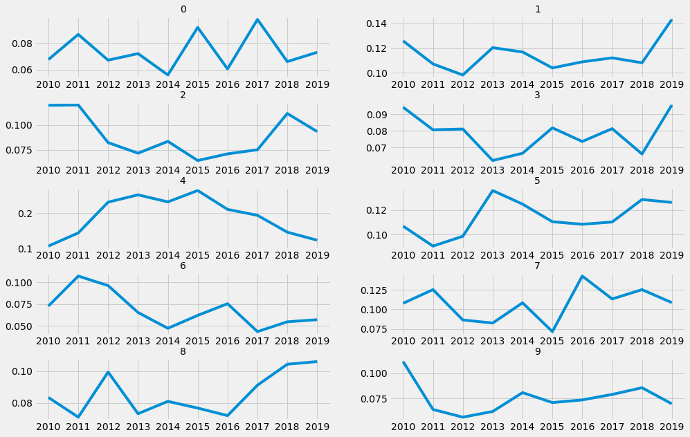
The following steps will build a figure with the evolution of each topic. These are calculated by evaluating the weight of each topic in the documents for a certain year and then summing up these weights.
evolution = np.zeros([len(corpus),10]) # We pre-build the numpy array filled with zeroes.
ind = 0
for bow in corpus:
    topics = lda_model.get_document_topics(bow)
    for topic in topics:
        evolution[ind,topic[0]] = topic[1]
    ind+=1
We create a pandas dataframe from the NumPy array and add the years and column names.
evolution_df = pd.DataFrame(evolution)
evolution_df['Year'] = file_years
evolution_df['Date'] = pd.to_datetime(evolution_df['Year'],format = "%Y") # Change Year to datetime-object.
evolution_df.set_index('Date',inplace=True) # Set Date as an index of the dataframe
evolution_df.drop('Year',axis=1,inplace = True)
plt.style.use('fivethirtyeight')
fig,axs = plt.subplots(5,2,figsize = [15,10])
for ax,column in zip(axs.flat,evolution_df.groupby('Date').mean().columns):
    ax.plot(evolution_df.groupby('Date').mean()[column])
    ax.set_title(column,{'fontsize':14})
plt.subplots_adjust(hspace=0.4)
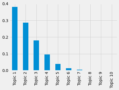
Next, we plot the marginal topic distribution, i.e., the relative importance of the topics. It is calculated by summing the topic weights of all documents.
First, we calculate the topic weights for every document.
doc_tops = []
for doc in corpus:
    doc_tops.append([item for (_,item) in lda_model.get_document_topics(doc)])
doc_tops_df = pd.DataFrame(doc_tops,columns=top_words_df.columns)
Then, we sum (and plot) these weights.
doc_tops_df = doc_tops_df/doc_tops_df.sum().sum()
doc_tops_df.sum(axis=0).plot.bar()
<matplotlib.axes._subplots.AxesSubplot at 0x7fca454fd2b0>
As our subsequent analysis, let’s search the most representative document for each topic. It is the document that has the largest weight for a certain topic.
doc_topics = []
for doc in corpus:
    doc_topics.append([item for (_,item) in lda_model.get_document_topics(doc)])
temp_df = pd.DataFrame(doc_topics)
With idxmax(), we can pick up the index that has the largest weight.
temp_df.idxmax()
0    1172
1    1775
2     858
3    1705
4    1644
5     133
6     517
7    1203
8     303
dtype: int64
We can now use files to connect indices to documents. For example, the most representative document of Topic 1 (index 0) is “PRACTICING SAFE COMPUTING: A MULTIMETHOD EMPIRICAL EXAMINATION OF HOME COMPUTER USER SECURITY BEHAVIORAL INTENTIONS”
files[1172]
'2010_2729.txt'
raw_text[1172][0:500]
'Anderson & Agarwal/Practicing Safe Computing\n\nSPECIAL ISSUE\n\nPRACTICING SAFE COMPUTING: A MULTIMETHOD EMPIRICAL EXAMINATION OF HOME COMPUTER USER SECURITY BEHAVIORAL INTENTIONS1\n\nBy: Catherine L. Anderson Decision, Operations, and Information Technologies Department Robert H. Smith School of Business University of Maryland Van Munching Hall College Park, MD 20742-1815 U.S.A. Catherine_Anderson@rhsmith.umd.edu\nRitu Agarwal Center for Health Information and Decision Systems Robert H. Smith School '
Let’s build a master table that has the document names and other information.
master_df = pd.DataFrame({'Article':files})
First, we add the most important topic of each article to the table.
top_topic = []
for doc in corpus:
    test=lda_model.get_document_topics(doc)
    test2 = [item[1] for item in test]
    top_topic.append(test2.index(max(test2))+1)

master_df['Top topic'] = top_topic
With head(), we can check the first (ten) values of our dataframe.
master_df.head(10)
| Article | Top topic | |
|---|---|---|
| 0 | 2019_1167.txt | 1 |
| 1 | 2017_27218.txt | 3 |
| 2 | 2012_40089.txt | 3 |
| 3 | 2012_2684.txt | 2 |
| 4 | 2015_16392.txt | 1 |
| 5 | 2019_3891.txt | 1 |
| 6 | 2011_1162.txt | 1 |
| 7 | 2015_19684.txt | 4 |
| 8 | 2010_2866.txt | 2 |
| 9 | 2018_30301.txt | 2 |
value_counts() for the “Top topic” -column can be used to check that in how many documents each topic is the most important.
master_df['Top topic'].value_counts()
1    794
2    604
3    402
4    210
5     81
6     23
7      9
9      2
8      1
Name: Top topic, dtype: int64
2.2. Summarisation
Let’s do something else. Gensim also includes efficient summarisation-functions (these are not related to LDA any more):
From the summarization -module, we can use summarize to automatically build a short summarisation of the document. Notice that we use the original documents for this and not the preprocessed ones. ratio = 0.01 means that the length of the summarisation should be 1 % from the original document.
summary = []
for file in raw_text:
    summary.append(gensim.summarization.summarize(file.replace('\n',' '),ratio=0.01))
Below is an example summary for the first document.
summary[1]
'*NLM Title Abbreviation:* J Appl Psychol *Publisher:* US : American Psychological Association *ISSN:* 0021-9010 (Print) 1939-1854 (Electronic) *ISBN:* 978-1-4338-9042-0 *Language:* English *Keywords:* ability, personality, interests, motivation, individual differences *Abstract:* This article reviews 100 years of research on individual differences and their measurement, with a focus on research published in the Journal of Applied Psychology.\nWe focus on 3 major individual differences domains: (a) knowledge, skill, and ability, including both the cognitive and physical domains; (b) personality, including integrity, emotional intelligence, stable motivational attributes (e.g., achievement motivation, core self-evaluations), and creativity; and (c) vocational interests.\n(PsycINFO Database Record (c) 2017 APA, all rights reserved) *Document Type:* Journal Article *Subjects:* *Individual Differences; *Measurement; *Motivation; *Occupational Interests; *Personality; Ability; Interests *PsycINFO Classification:* Occupational & Employment Testing (2228) Occupational Interests & Guidance (3610) *Population:* Human *Tests & Measures:* Vocational Preference Inventory *Methodology:* Literature Review *Supplemental Data:* Tables and Figures Internet *Format Covered:* Electronic *Publication Type:* Journal; Peer Reviewed Journal *Publication History:* First Posted: Feb 2, 2017; Accepted: Jun 27, 2016; Revised: Jun 2, 2016; First Submitted: Aug 12, 2015 *Release Date:* 20170202 *Correction Date:* 20170309 *Copyright:* American Psychological Association.\n85) The development of standardized measures of attributes on which individuals differ emerged very early in psychology’s history, and has been a major theme in research published in the /Journal of Applied Psychology/ (/JAP/).\nThus, ability, personality, interest patterns, and motivational traits (e.g., achievement motivation, core self-evaluations [CSEs]) fall under the individual differences umbrella, whereas variables that are transient, such as mood, or that are closely linked to the specifics of the work setting (e.g., turnover intentions or perceived organizational climate), do not.\nThe very first volume of the journal contained research on topics that are core topics of research today, including criterion-related validity (Terman et al., 1917 <#c252>), bias and group differences (Sunne, 1917 <#c245>), measurement issues (Miner, 1917 <#c181>; Yerkes, 1917 <#c282>), and relationships with learning and the development of knowledge and skill (Bingham, 1917 <#c26>).\nOver the years, studies have reflected the tension between viewing cognitive abilities as enduring capacities that are largely innate versus treating them as measures of developed capabilities, a distinction that has implications for the study of criterion related validity, group differences, aging effects, and the structure of human abilities (Kuncel & Beatty, 2013 <#c155>).\nIn addition to the direct study of knowledge and skill measurement, these individual differences have been a part of research on job analysis, leadership, career development, performance appraisal, training, and skill acquisition, among others.\nIn a well-cited /JAP/ article, Ghiselli and Barthol (1953) <#c94> summarized this first era by reviewing 113 studies about the validity of personality inventories for predicting job performance.\nBy using only measures designed to assess the FFM, Hurtz and Donovan’s (2000) <#c129> meta-analysis addressed potential construct-related validity concerns of prior meta-analyses and found evidence for personality as a predictor of task and contextual performance.\nSeveral meta-analyses, large-scale studies, and simulations were published in /JAP/ that demonstrated the limited impact of socially desirable responding and faking on the construct-related and criterion-related validity of personality measures (Ellingson, Smith, & Sackett, 2001 <#c66>; Ones, Viswesvaran, & Reiss, 1996 <#c200>; and, later on, Hogan, Barrett, & Hogan, 2007 <#c112>; Schmitt & Oswald, 2006 <#c229>).\nIn /JAP/, research has also appeared measuring personality with conditional reasoning tests (Bing et al., 2007 <#c25>), SJTs (Motowidlo, Hooper, & Jackson, 2006 <#c185>), structured interviews (Van Iddekinge, Raymark, & Roth, 2005 <#c268>), and ideal point models (Stark, Chernyshenko, Drasgow, & Williams, 2006 <#c240>), though not all of these approaches demonstrated incremental prediction over self-reports.\nSome of the more notable advancements are that (a) personality can interact with the situation to affect behavior (e.g., Tett & Burnett’s [2003] <#c253> trait activation theory); (b) motivational forces mediate the effects of personality (e.g., Barrick, Stewart, & Piotrowski, 2002 <#c18>), with both implicit and explicit motives being important (Frost, Ko, & James, 2007 <#c86>; Lang, Zettler, Ewen, & Hülsheger, 2012 <#c157>); (c) personality is stable, yet also prone to change, across life (Woods & Hampson, 2010 <#c279>); (d) personality both affects and is affected by work (Wille & De Fruyt, 2014 <#c275>); and (e) personality traits represent stable distributions of variable personality states (Judge, Simon, Hurst, & Kelley, 2014 <#c147>; Minbashian, Wood, & Beckmann, 2010 <#c180>).\n/JAP/ has published several articles that have contributed to the understanding of integrity tests, including Hogan and Hogan (1989) <#c113> on the measurement of employee reliability, and studies that examined faking (Cunningham, Wong, & Barbee, 1994 <#c51>), subgroup differences (Ones & Viswesvaran, 1998 <#c199>), and difficulties in predicting low base rate behaviors (Murphy, 1987 <#c188>).\nIt is worth noting that other individual difference measures have also been examined in /JAP/ as predictors of CWB, including biodata (Rosenbaum, 1976 <#c217>), conditional reasoning (Bing et al., 2007 <#c25>; LeBreton, Barksdale, Robin, & James, 2007 <#c161>), and the Big Five personality dimensions (Berry, Ones, & Sackett, 2007 <#c22>).\nFourth, many studies during this period focused on the vocational interests of particular groups or of individuals in specific jobs or occupations, including tuberculosis patients (Shultz & Rush, 1942 <#c235>), industrial psychology students (Lawshe & Deutsch, 1952 <#c159>), retired YMCA secretaries (Verburg, 1952 <#c271>), and female computer programmers (Perry & Cannon, 1968 <#c206>).'
master_df['Summaries'] = summary
master_df
| Article | Top topic | Summaries | |
|---|---|---|---|
| 0 | 2019_1167.txt | 1 | We add to the literature on the economics of c... |
| 1 | 2017_27218.txt | 3 | *NLM Title Abbreviation:* J Appl Psychol *... |
| 2 | 2012_40089.txt | 3 | Service Quality in Software-as-a-Service: Deve... |
| 3 | 2012_2684.txt | 2 | RESEARCH ARTICLE UNDERSTANDING USER REVISIONS... |
| 4 | 2015_16392.txt | 1 | *Document Type:* Article *Subject Terms:* ... |
| ... | ... | ... | ... |
| 2121 | 2016_2942.txt | 1 | {rajiv.kohli@mason.wm.edu} Sharon Swee-Lin Tan... |
| 2122 | 2016_81.txt | 2 | J Bus Ethics (2016) 138:349364 DOI 10.1007/s10... |
| 2123 | 2018_13221.txt | 6 | Sinha Carlson School of Management, University... |
| 2124 | 2016_23236.txt | 1 | *Document Type:* Article *Subject Terms:* ... |
| 2125 | 2016_38632.txt | 4 | To understand the trade-offs involved in decid... |
2126 rows × 3 columns
The same summarization -module also includes a function to search keywords from the documents. It works in the same way as summarize().
keywords = []
for file in raw_text:
    keywords.append(gensim.summarization.keywords(file.replace('\n',' '),ratio=0.01).replace('\n',' '))
Here are keywords for the second document
keywords[1]
'journal journals psychology psychological personality person personal research researchers researched performance performing perform performed performances testing tests test tested measurement measures measureable measure measured measuring ability abilities difference different differing differs study studies studied individual differences individuals differ job jobs interests interesting interested including include includes included traits trait'
master_df['Keywords'] = keywords
master_df
| Article | Top topic | Summaries | Keywords | |
|---|---|---|---|---|
| 0 | 2019_1167.txt | 1 | We add to the literature on the economics of c... | bitcoin bitcoins user users transactions trans... |
| 1 | 2017_27218.txt | 3 | *NLM Title Abbreviation:* J Appl Psychol *... | journal journals psychology psychological pers... |
| 2 | 2012_40089.txt | 3 | Service Quality in Software-as-a-Service: Deve... | service services saas research researchers cus... |
| 3 | 2012_2684.txt | 2 | RESEARCH ARTICLE UNDERSTANDING USER REVISIONS... | use uses usefulness features feature user user... |
| 4 | 2015_16392.txt | 1 | *Document Type:* Article *Subject Terms:* ... | automation automated automate work working hum... |
| ... | ... | ... | ... | ... |
| 2121 | 2016_2942.txt | 1 | {rajiv.kohli@mason.wm.edu} Sharon Swee-Lin Tan... | data ehr ehrs research researchers health pati... |
| 2122 | 2016_81.txt | 2 | J Bus Ethics (2016) 138:349364 DOI 10.1007/s10... | organizational relationship relationships altr... |
| 2123 | 2018_13221.txt | 6 | Sinha Carlson School of Management, University... | firms firm production product products modelin... |
| 2124 | 2016_23236.txt | 1 | *Document Type:* Article *Subject Terms:* ... | reviewer reviews review reviewers reviewed rev... |
| 2125 | 2016_38632.txt | 4 | To understand the trade-offs involved in decid... | time timing hire hiring hired management manag... |
2126 rows × 4 columns
2.3. Similarities
As a next example, we analyse the similarities between the documents.
Gensim has a specific function for that: SparseMatrixSimilarity
from gensim.similarities import SparseMatrixSimilarity
The parameters to the function are the word-frequency corpus and the length of the dictionary.
index = SparseMatrixSimilarity(corpus,num_features=len(id2word))
sim_matrix = index[corpus]
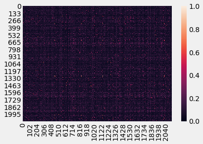
In the similarity matrix, the diagonal has values 1 (similarity of a document with itself). We replace those values with zero to find the most similar documents from the corpus.
for i in range(len(sim_matrix)):
    sim_matrix[i,i] = 0
Seaborn (https://seaborn.pydata.org/) has a convenient heatmap function to plot similarities. Here is information about Seaborn from their web page: Seaborn is a Python data visualization library based on Matplotlib. It provides a high-level interface for drawing attractive and informative statistical graphics.
sns.heatmap(sim_matrix)
<matplotlib.axes._subplots.AxesSubplot at 0x7fca4c47e6d0>
We search the most similar article by locating the index with a largest value for every column.
master_df['Most_similar_article'] = np.argmax(sim_matrix,axis=1)
master_df
| Article | Top topic | Summaries | Keywords | Most_similar_article | |
|---|---|---|---|---|---|
| 0 | 2019_1167.txt | 1 | We add to the literature on the economics of c... | bitcoin bitcoins user users transactions trans... | 1306 |
| 1 | 2017_27218.txt | 3 | *NLM Title Abbreviation:* J Appl Psychol *... | journal journals psychology psychological pers... | 2090 |
| 2 | 2012_40089.txt | 3 | Service Quality in Software-as-a-Service: Deve... | service services saas research researchers cus... | 28 |
| 3 | 2012_2684.txt | 2 | RESEARCH ARTICLE UNDERSTANDING USER REVISIONS... | use uses usefulness features feature user user... | 1796 |
| 4 | 2015_16392.txt | 1 | *Document Type:* Article *Subject Terms:* ... | automation automated automate work working hum... | 1280 |
| ... | ... | ... | ... | ... | ... |
| 2121 | 2016_2942.txt | 1 | {rajiv.kohli@mason.wm.edu} Sharon Swee-Lin Tan... | data ehr ehrs research researchers health pati... | 301 |
| 2122 | 2016_81.txt | 2 | J Bus Ethics (2016) 138:349364 DOI 10.1007/s10... | organizational relationship relationships altr... | 2070 |
| 2123 | 2018_13221.txt | 6 | Sinha Carlson School of Management, University... | firms firm production product products modelin... | 1942 |
| 2124 | 2016_23236.txt | 1 | *Document Type:* Article *Subject Terms:* ... | reviewer reviews review reviewers reviewed rev... | 1917 |
| 2125 | 2016_38632.txt | 4 | To understand the trade-offs involved in decid... | time timing hire hiring hired management manag... | 412 |
2126 rows × 5 columns
2.4. Cluster model
Next, we build a topic analysis using a different approach. We create a TF-IDF model from the corpus and apply K-means clustering for that model.
Explanation of TF-IDF from Wikipedia: “In information retrieval, TF–IDF or TFIDF, short for term frequency–inverse document frequency, is a numerical statistic that is intended to reflect how important a word is to a document in a collection or corpus. It is often used as a weighting factor in searches of information retrieval, text mining, and user modelling. The TF–IDF value increases proportionally to the number of times a word appears in the document and is offset by the number of documents in the corpus that contain the word, which helps to adjust for the fact that some words appear more frequently in general.”
Explanation of K-means clustering from Wikipedia: “k-means clustering is a method of vector quantization, originally from signal processing, that aims to partition n observations into k clusters in which each observation belongs to the cluster with the nearest mean (cluster centres or cluster centroid), serving as a prototype of the cluster…k-means clustering minimizes within-cluster variances (squared Euclidean distances)…”
From Gensim.models we pick up TfidModel.
from gensim.models import TfidfModel
As parameters, we need the corpus and the dictionary.
tf_idf_model = TfidfModel(corpus,id2word=id2word)
We use the model to build up a TF-IDF -transformed corpus.
tform_corpus = tf_idf_model[corpus]
corpus2csc converts a streamed corpus in bag-of-words format into a sparse matrix, with documents as columns.
spar_matr = gensim.matutils.corpus2csc(tform_corpus)
spar_matr
<32237x2126 sparse matrix of type '<class 'numpy.float64'>'
	with 1897708 stored elements in Compressed Sparse Column format>
Sparse matrix to normal array. Also, we need to transpose it for the K-means model.
tfidf_matrix = spar_matr.toarray().transpose()
tfidf_matrix
array([[0.00125196, 0.00243009, 0.00474072, ..., 0.        , 0.        ,
        0.        ],
       [0.        , 0.00594032, 0.        , ..., 0.        , 0.        ,
        0.        ],
       [0.        , 0.        , 0.        , ..., 0.        , 0.        ,
        0.        ],
       ...,
       [0.        , 0.0077254 , 0.        , ..., 0.        , 0.        ,
        0.        ],
       [0.00396927, 0.        , 0.        , ..., 0.        , 0.        ,
        0.        ],
       [0.        , 0.        , 0.        , ..., 0.        , 0.        ,
        0.        ]])
tfidf_matrix.shape
(2126, 32237)
Scikit-learn has a function to form a K-means clustering model from a matrix. It is done below. We use ten clusters.
from sklearn.cluster import KMeans

kmodel = KMeans(n_clusters=10)

kmodel.fit(tfidf_matrix)

clusters = km.labels_.tolist()
master_df['Tf_idf_clusters'] = clusters
km.cluster_centers_
array([[ 1.33476883e-03,  4.71424426e-03,  2.62007897e-04, ...,
         2.71050543e-20,  3.38813179e-21,  0.00000000e+00],
       [ 6.67748803e-04,  9.98513608e-04,  9.39093177e-04, ...,
         1.00166900e-03,  6.77626358e-21,  5.77802403e-05],
       [ 1.96181867e-04,  3.44260097e-04,  1.83757076e-04, ...,
        -5.42101086e-20,  0.00000000e+00, -3.38813179e-21],
       ...,
       [ 0.00000000e+00,  3.26892198e-03,  1.67826509e-03, ...,
        -8.13151629e-20, -1.69406589e-21, -3.38813179e-21],
       [ 5.84538250e-04,  1.55948712e-03,  2.28571545e-04, ...,
         0.00000000e+00, -3.38813179e-21, -3.38813179e-21],
       [ 5.10233572e-04,  4.11021862e-03,  1.24048649e-03, ...,
        -2.71050543e-20,  1.69406589e-21, -3.38813179e-21]])
master_df
| Article | Top topic | Summaries | Keywords | Most_similar_article | Tf_idf_clusters | |
|---|---|---|---|---|---|---|
| 0 | 2019_1167.txt | 1 | We add to the literature on the economics of c... | bitcoin bitcoins user users transactions trans... | 1306 | 5 |
| 1 | 2017_27218.txt | 3 | *NLM Title Abbreviation:* J Appl Psychol *... | journal journals psychology psychological pers... | 2090 | 4 |
| 2 | 2012_40089.txt | 3 | Service Quality in Software-as-a-Service: Deve... | service services saas research researchers cus... | 28 | 4 |
| 3 | 2012_2684.txt | 2 | RESEARCH ARTICLE UNDERSTANDING USER REVISIONS... | use uses usefulness features feature user user... | 1796 | 4 |
| 4 | 2015_16392.txt | 1 | *Document Type:* Article *Subject Terms:* ... | automation automated automate work working hum... | 1280 | 2 |
| ... | ... | ... | ... | ... | ... | ... |
| 2121 | 2016_2942.txt | 1 | {rajiv.kohli@mason.wm.edu} Sharon Swee-Lin Tan... | data ehr ehrs research researchers health pati... | 301 | 8 |
| 2122 | 2016_81.txt | 2 | J Bus Ethics (2016) 138:349364 DOI 10.1007/s10... | organizational relationship relationships altr... | 2070 | 4 |
| 2123 | 2018_13221.txt | 6 | Sinha Carlson School of Management, University... | firms firm production product products modelin... | 1942 | 5 |
| 2124 | 2016_23236.txt | 1 | *Document Type:* Article *Subject Terms:* ... | reviewer reviews review reviewers reviewed rev... | 1917 | 5 |
| 2125 | 2016_38632.txt | 4 | To understand the trade-offs involved in decid... | time timing hire hiring hired management manag... | 412 | 5 |
2126 rows × 6 columns
Let’s collect the ten most important words for each cluster.
centroids = km.cluster_centers_.argsort()[:, ::-1] # Sort the words according to their importance.

for i in range(num_clusters):
    j=i+1
    print("Cluster %d words:" % j, end='')
    for ind in centroids[i, :10]:
        print(' %s' % id2word.id2token[ind],end=',')
    print()
    print()
Cluster 1 words: patent, movie, tweet, invention, citation, inventor, innovation, twitter, follower, release,

Cluster 2 words: analytic, innovation, digital, capability, governance, supply_chain, sustainability, right_reserve, big, platform,

Cluster 3 words: persistent_linking, site_ehost, true_db, learning_please, academic_licensee, syllabus_mean, newsletter_content, electronic_reserve, authorize_ebscohost, course_pack,

Cluster 4 words: auction, bidder, bid, advertiser, bidding, price, pricing, combinatorial_auction, seller, valuation,

Cluster 5 words: team, employee, job, organizational, project, ethic, security, task, member, community,

Cluster 6 words: consumer, privacy, web_delivery, rating, disclosure, investor, participant, website, app, wom,

Cluster 7 words: brand, marketing, retailer, consumer, advertising, purchase, marketer, elasticity, promotion, sale,

Cluster 8 words: optimization, optimal, theorem, algorithm, node, approximation, scheduling, constraint, parameter, distribution,

Cluster 9 words: patient, hospital, physician, care, healthcare, medical, clinical, hit, health, health_care,

Cluster 10 words: price, inventory, retailer, supplier, pricing, contract, profit, demand, forecast, optimal,
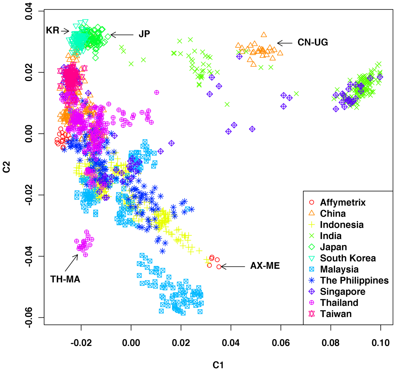
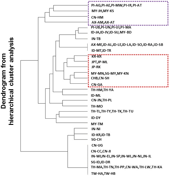
With a smaller corpus, we could use fancy visualisations, like multidimensional scaling and Ward-clustering, to represent the document relationship. However, with over 2000 documents, that is not meaningful. Below are examples of both (not related to our analysis).
With pandas crosstab, we can easily check the connection between the LDA topics and the K-means clusters.
pd.crosstab(master_df['Top topic'],master_df['Tf_idf_clusters'])
| Tf_idf_clusters | 0 | 1 | 2 | 3 | 4 | 5 | 6 | 7 | 8 | 9 |
|---|---|---|---|---|---|---|---|---|---|---|
| Top topic | ||||||||||
| 1 | 14 | 151 | 91 | 10 | 175 | 157 | 28 | 77 | 32 | 59 |
| 2 | 10 | 122 | 44 | 13 | 138 | 124 | 21 | 37 | 39 | 56 |
| 3 | 7 | 79 | 21 | 4 | 76 | 114 | 15 | 25 | 18 | 43 |
| 4 | 5 | 30 | 6 | 1 | 31 | 84 | 16 | 8 | 9 | 20 |
| 5 | 1 | 8 | 0 | 2 | 12 | 34 | 6 | 2 | 7 | 9 |
| 6 | 1 | 1 | 0 | 1 | 2 | 13 | 0 | 0 | 2 | 3 |
| 7 | 0 | 0 | 0 | 0 | 2 | 6 | 0 | 0 | 0 | 1 |
| 8 | 0 | 1 | 0 | 0 | 0 | 0 | 0 | 0 | 0 | 0 |
| 9 | 0 | 0 | 0 | 0 | 1 | 0 | 0 | 0 | 0 | 1 |